Bridson's Blue Noise Algorithm Examined
Finding a realistic (or at least, realistic looking) initial configuration of game objects or simulation particles can be a challenge. The desired configuration should appear to be both “random” and at the same time “spatially uniform”, without objects clustering together or overlapping.
(The problem is, by the way, not limited to games: when simulating particle systems, such as liquids, finding a realistic initial configuration can be a real challenge, as well.)
It is not obvious how to achieve a satisfactory configuration. Placing items manually will lead to the same configuration on every run, and is infeasible when the number of objects grows large anyway. The two trivial computational approaches both fall flat as well, in different ways: putting items on a grid is not random, and placing items randomly does not prevent undesirable clustering or even overlap of objects.
An algorithm that is often recommended to generate satisfactory configurations is Bridson’s Algorithm. The algorithm is both short (the paper introducing it is quite literally a one-pager) and fast. It clearly works (in some way — see the figures on this page); yet, having implemented it, I realized that the algorithm does not quite do what I expected it to do. It solves a different problem from the one I thought it did.
Summary
The algorithm grows a random cluster with a fixed average density of points.
The algorithm does not place points randomly into the entire extent of a box, while maintaining a given minimum-distance constraint. If the number of points is too small, the generated cluster will not fill the box.
The resulting configuration is much less random than may be expected; the typical distance between neighbors is nearly constant (and hence not very random at all). The algorithm does not produce configurations such that some points are close together and others are further apart.
Good results may be obtained by drawing a smaller random sample from a set of positions generated by the original algorithm.
All these facts may, of course, be acceptable (or even desirable!) for a given application. But one should be clear about the amount of “randomness” (or the lack thereof) in the point configurations that are created when using this algorithm.
The Algorithm
Informally, the algorithm starts by placing an initial game object. The algorithm then attempts to place another game object randomly in the vicinity of one of the existing objects, but without coming too close to an existing object. The algorithm continues until the desired number of items has been placed. The algorithm makes use of an auxiliary grid data structure to speed up the neighborhood evaluations.
More formally, and adapted pretty directly from Gridson’s paper:
-
There is really only one adjustable input parameter, namely the minimum distance between points
rthat must be chosen prior to running the algorithm. -
Initialize an d-dimensional background grid for storing samples and accelerating spatial searches. The cell size (measured along one of the coordinate axes!) should be less than $r/\sqrt{d}$, where $d$ is the dimensionality of the space. This ensures that the cells are so small that each cell will be occupied by at most one point. (The factor of $1/\sqrt{d}$ is simply the length of the space diagonal of the d-dimensional unit hypercube: it is the usual Euclidean length of the vector $(1, 1, \dots, 1)$.)
-
Place an initial point anywhere in the grid. (The original paper says to place this point randomly in the simulation box; for reasons that will be discussed later, it should be placed near the box’s center. In fact, little harm is done by putting it deterministically at the center position.) Also add this point to the list of active points.
-
Repeat the following steps until either the active list is empty, or the desired number of points has been generated:
- Pick a point
x0, y0randomly from the active list. - Make several attempts (typically up to 30 or so) to place a new
point
x, yrandomly into the annulus between radiusrand2*raroundx0, y0. Accept the first such point that is not within distancerof one of the existing points. (It is necessary to examine the grid cell containing the new pointx, y, as well as all the cells surrounding it, to check for conflicts.) - If an acceptable point has been found, add it to both the list and the cell.
- If no acceptable point has been found after the allotted number
of attempts, remove the initial point
x0, y0from the active list. - Iterate (by picking a new point
x0, y0from the active list).
- Pick a point
The Implementation
Below is my implementation of Gridson’s Algorithm (for two dimensions only — generalization to d dimensions is straightforward). It follows the specification fairly literally. One difference is that I don’t actually create the “grid” as a two dimensional data structure, because I expect most of the cells to be empty, anyway. Instead, I merely calculate the indices of the grid cell for a particle, and then use them as keys into a hashmap (dictionary). This design preserves the essential feature, which is that one can generate the indices of the neighboring cells, in order to iterate over them.
Another difference to the published algorithm is that I make provisions to restrict the generated positions to fall inside the simulation box. This can be done either by using periodic boundary conditions, or by rejecting positions outside the box. (The published article lists width and height of the box as inputs, but does not refer to them in any way later on.)
def blue_noise_2d( width, height, min_dist, samples,
                   max_trials=30, bdry_conds="fixed" ):
    grid = {}
    list = []
    bin = min_dist/math.sqrt(2.0)

    # Place initial point in grid and list:
    # x, y = random.uniform( 0, width ), random.uniform( 0, height )
    x, y = width/2, height/2
    grid[ ( int(x/bin), int(y/bin) ) ] = (x,y)
    list.append( (x,y) )

    # Loop until list is empty:
    while len(list):

        # Pick random point from list:
        k = random.randrange( len(list) )
        ( x0, y0 ) = list[k]

        # Trials to place the next point:
        for trial in range( max_trials ):

            # Generate a trial point in annulus r..2*r around x0,y0
            r = random.uniform( min_dist, 2.0*min_dist )
            phi = random.uniform( 0, 2.0*math.pi )
            x, y = x0 + r*math.cos(phi), y0 + r*math.sin(phi)

            if bdry_conds == "fixed":
                # Reject point if outside the boundaries
                if not (0 <= x <= width and 0 <= y <= height ):
                    continue
            else:
                # Enforce periodic bdry conds
                x, y = math.fmod(width+x, width), math.fmod(height+y, height)

            # Find the grid cell of trial point
            i, j = int(x/bin), int(y/bin)

            # Iterate over neighbors, looking for conflicts w/ occupied nbs
            conflict = False
            for u in [-1, 0, 1]:
                for v in [-1, 0, 1]:
                    if (i+u, j+v) in grid:
                        conflict = True
                        break

            # if no conflict, accept trial pt into grid and list, stop trials
            if not conflict:
                grid[ (i, j) ] = (x, y)
                list.append( (x, y) )
                break

        # loop-else: gone through all trials without success: rm initial pt
        else:
            list.pop(k)

        # Stop if enough points generated
        if len(grid.keys()) >= samples:
            break

    return grid
The implementation uses two Python-specific features:
-
A tuple is a valid hash key, hence I can use a tuple of bin indices
(i,j)directly as key and don’t have to transform it into (say) a string. -
The implementation gave me an opportunity to use Python’s “loop-else” (for the first time, ever!): a block that will be executed only if the loop has run to completion, and has not been interrupted through a
breakstatement. (This avoids the use of asuccessflag that would be only set toTruein theif not conflict:block.)
Examples and Surprises
I must admit that the description of the algorithm (and even the implementation) did not give me a good intuitive sense for “how the algorithm works”. Running a few test runs was therefore very illuminating — but also surprising (and not really in a good way).
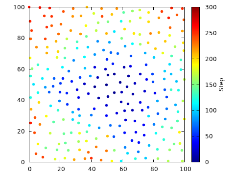
The following figure shows a 100x100 box, with the minimum distance r=4.
The initial point was placed at (50,50).
The algorithm was run until the “active list” of growth centers was
empty. The final number of points placed is 259.
The points have been colored to indicate when they were placed. It is obvious that the points were added, fairly continuously, from the center out. New points tended to be added at the perimeter of the region already containing points.
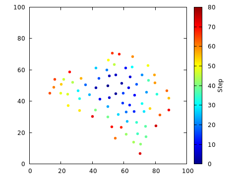
To make this argument more clearly, in the following figure, the algorithm was stopped after 75 samples where placed. Clearly, the points do not fill the box; instead, they form a cluster of known density.
This is not what I wanted. I need only 30 points, but I want them to
fill the box. This can be achieved by increasing the minimum distance
accordingly; for r=12, I obtained the following configuration (of
31 points, to be exact).

Now the points fill the box, but the minimum observed distance is unnecessarily (and, for the intended application) undesirably large.
In fact, it can be difficult, using the present algorithm, to get a specific number of points into a fixed box. For random graphics, this is a non-issue, for games or particle simulations, it is often more serious.
Problem Solved: Subsampling for Randomness
One (trivial) modification of the original algorithm that I have
found useful for my own purposes is to take a random sample from
the points generated by the algorithm. Essentially, I chose a desirable
minimum distance, and then let the algorithm generate as many points as
it can fit into the box. From this set of points, I then chose randomly
a much smaller sample of positions. These will still obey the desired
minimum distance constraint, but be essentially “randomly” distributed
throughout the simulation box. (The constant density of generated points
helps here: no region of the box is in some way preferred over any other.)
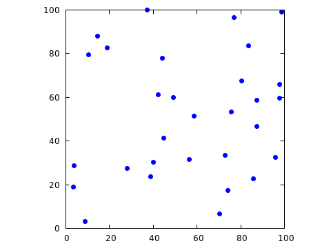
It is now also no problem to create a random sample containing exactly
the desired number of points! Here is the result when choosing 30 points
from the initial sample with r=4.
Discussion
Bridson’s algorithm is nice, but it seems more suitable for generating random, but uniform “textures”, rather than space-filling, random configurations one might want in a game. Drawing a smaller, random sample from the set of generated positions, as described in the previous section, does lead to good results, though.
In fact, it seems to me that a possible application area of the algorithm is to create starting configurations for simulations of dense liquids. It is notoriously difficult to create good starting configurations for such simulations; the ad-hoc methods used typically used either give results that are much worse than the current algorithm, or much more complicated. A recent (2017) standard reference recommends an approach amounting to simulated annealing — surely overkill compared to the present algorithm!
Resources
-
Why is it called “blue noise”? Wikipedia has the answer.