The Diamond-Square Algorithm for Terrain Generation

The Diamond-Square Algorithm is the natural first stop for generating artificial landscapes. The algorithm itself is beautifully simple (more details below, and on its Wikipedia page). But a casual implementation ended up not working at all, prompting me to look for an existing implementation to learn from. However, most implementations I found looked hideously complicated (or just hideous), not necessarily correct, and/or used out-of-date programming languages and styles. It therefore seemed like a good idea to create a clean, simple “reference” implementation of this algorithm, using a contemporary and widely known programming language and style.

The Diamond-Square Algorithm

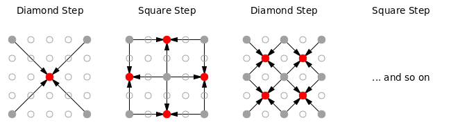
The Diamond-Square Algorithm successively populates an n-by-n array, at increasing level of detail. Initially, only the corners need to be initialized; the remaining cells in the array are then populated by averaging over the four nearest populated neighbors, and adding a small random amount.

• The algorithm requires that the edge length of the array is one greater than an integer power of two: n = 1+2**k, where k is a positive integer.
• At each step, the amplitude of the random noise is reduced by some factor. The smaller the factor, the smoother the resulting landscape.
• There are two possibilities to deal with pixels laying on the edge of the array: using “fixed” boundary conditions, the average is performed only over the populated cells that lie within the array. Using “periodic” boundary conditions, the averaging routine “wraps around” and pulls in values from the opposite site of the array.

The algorithm feels recursive, but isn’t really. Because the value assigned to each cell depends on the cell’s neighbors, the problem does not partition into a smaller version of itself, and it is more natural to process the entire field at each step, but at increasing level of detail.

Implementation

Here is a Python implementation of the Diamond-Square algorithm.

The entry point is the make_terrain() function, which manages the iteration over the decreasing cell sizes, until all pixels have been filled in. It returns a populated np.array.

The make_terrain() function calls the single_diamond_square_step() routine, which performs first a diamond step, followed by a square step. The square step is broken into two passes: one fills in the even-numbered rows, the other the even-numbered columns.

The actual averages over the four neighbors is performed by one of the two functions fixed() or periodic(). In addition to the actual averaging, they also contain logic to handle the boundary conditions.

The implementation does not initialize the seed values at the four corners to user-supplied values; instead, they are all set to zero. (This could be changed easily.) Notice that for periodic boundary conditions, all four corners represent the same pixel and therefore should be set to the same value.

import random
import numpy as np

def fixed( d, i, j, v, offsets ):
    # For fixed bdries, all cells are valid. Define n so as to allow the
    # usual lower bound inclusive, upper bound exclusive indexing.
    n = d.shape[0]
    
    res, k = 0, 0
    for p, q in offsets:
        pp, qq = i + p*v, j + q*v
        if 0 <= pp < n and 0 <= qq < n:
            res += d[pp, qq]
            k += 1.0
    return res/k

def periodic( d, i, j, v, offsets ):
    # For periodic bdries, the last row/col mirrors the first row/col.
    # Hence the effective square size is (n-1)x(n-1). Redefine n accordingly!
    n = d.shape[0] - 1
    
    res = 0
    for p, q in offsets:
        res += d[(i + p*v)%n, (j + q*v)%n]
    return res/4.0
            
def single_diamond_square_step( d, w, s, avg ):
    # w is the dist from one "new" cell to the next
    # v is the dist from a "new" cell to the nbs to average over
    
    n = d.shape[0]
    v = w//2
    
    # offsets:
    diamond = [ (-1,-1), (-1,1), (1,1), (1,-1) ]
    square = [ (-1,0), (0,-1), (1,0), (0,1) ]

    # (i,j) are always the coords of the "new" cell

    # Diamond Step
    for i in range( v, n, w ):
        for j in range( v, n, w ):
            d[i, j] = avg( d, i, j, v, diamond ) + random.uniform(-s,s)
            
    # Square Step, rows
    for i in range( v, n, w ):
        for j in range( 0, n, w ):
            d[i, j] = avg( d, i, j, v, square ) + random.uniform(-s,s)

    # Square Step, cols
    for i in range( 0, n, w ):
        for j in range( v, n, w ):
            d[i, j] = avg( d, i, j, v, square ) + random.uniform(-s,s)
            
def make_terrain( n, ds, bdry ):
    # Returns an n-by-n landscape using the Diamond-Square algorithm, using 
    # roughness delta ds (0..1). bdry is an averaging fct, including the
    # bdry conditions: fixed() or periodic(). n must be 1+2**k, k integer.
    d = np.zeros( n*n ).reshape( n, n )
   
    w, s = n-1, 1.0
    while w > 1:
        single_diamond_square_step( d, w, s, bdry )

        w //= 2
        s *= ds

    return d

Using the Algorithm

Here is an example how this algorithm might be called.

n = 1 + 2**9    # Edge size of the resulting image in pixes
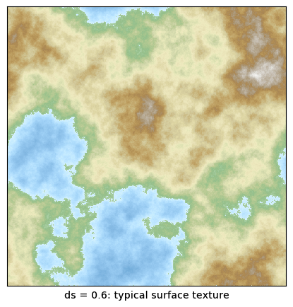
ds = 0.6        # Roughness delta, 0 < ds < 1 : smaller ds => smoother results
bdry = periodic # One of the averaging routines: fixed or periodic

terrain = make_terrain( n, ds, bdry )

The terrain variable contains a populated n-by-n array, which now can be rendered in some fashion. Here is an example that uses matplotlib’s imshow() function to create a heatmap version of the terrain. The resulting image can be saved to file (with savefig()) or rendered to the screen (using show()).

import matplotlib.colors
import matplotlib.pyplot as plt

# Create a colormap
tmp = []
for row in np.loadtxt( "geo-smooth.gpf" ):
    tmp.append( [ row[0], row[1:4] ] )
cm = matplotlib.colors.LinearSegmentedColormap.from_list( "geo-smooth", tmp )

# Create an image using the colormap
plt.figure( figsize=( n/100, n/100 ), dpi=100 ) # create n-by-n pixel fig
plt.tick_params( left=False, bottom=False, labelleft=False, labelbottom=False )
plt.imshow( terrain, cmap=cm )

plt.savefig( "terrain.png" )  # Save to file
plt.show()                    # Show interactive

The realistic appearance of the final image depends pretty critically on the colormap chosen to create the image. In fact, using a generic false-color palette, the resulting image does not evoke the impression of a “landscape” at all!

The file geo-smooth.gpf contains a palette suitable for topographic maps. All color transitions are smooth, with the exception of the one from “sea” to “land”, which is sharp, hence giving rise to sharp “coast lines” in the final image.

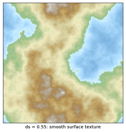
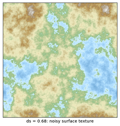
The roughness of the generated landscape is controlled by the roughness parameter ds. I have obtained good results with values of ds between about 0.55 (smooth) and 0.7 (noisy). Below are two typical examples.

Resources

• diamond-square.py
• geo-smooth.gpf