Heat Flow

Imagine a rod that is initially at temperature $T_1$ and then brought into an environment with a lower temperature $T_0 < T_1$. How quickly does the body cool down? When will it have reached the environment’s temperature? What is the temperature profile throughout the rod, as a function of time?

This is essentially a worked homework set: a complete, step-by-step solution of the diffusion (or heat) equation in one dimension.

Exact Solution

This problem is governed by the Diffusion or Heat Equation:

$$ \frac{\partial}{\partial t} T = D \nabla^2 T $$

with initial condition:

$$ T(x, t=0) = T_1 $$

and boundary condition:

$$ T(x=\pm L, t) = T_0 $$

FIGURE!

Separation of Variables

Separation ansatz:

$$ T(x,t) = U(t) \, V(x) $$

In the differential equation:

$$ \dot{U} \, V = D \, U \, V^{\prime \prime} $$

Divide by $T(x,t) = U(t) \, V(x)$:

$$ \frac{ \dot{U} }{U} = D \frac{ V^{\prime \prime} }{ V } = -C $$

where $C$ is an (as yet undetermined) constant. (The choice of sign will turn out to be convenient later.)

Note that $D$ has dimension $\text{length}^2/\text{time}$ and $C$ has dimension $1/\text{time}$.

The Temporal Equation

$$ \dot{U}(t) + C \, U(t) = 0 \qquad \text{with $U(t=0) = T_1$} $$

Solution:

$$ U(t) = T_1 \, e^{-C t} $$

Physically meaningful (decaying) behavior requires the constant to be positive: $C > 0$.

The Spatial Equation

$$ V^{\prime \prime}(x) + \frac{C}{D} V(x) = 0 $$

The original boundary condition is inhomogeneous:

$$ V(x=\pm L) = T_0 $$

We will first solve the equation subject to the homogeneous boundary condition $V(x=\pm L) = 0$ and later add the “particular” solution $V_0(x) = T_0$ to the general solution to take the original boundary condition into account.

The symmetry of the problem suggests that the solution will be even. Hence, solutions to the equation with homogeneous boundary condition are of the form (where $A_n$ are undetermined amplitudes):

$$ V_n(x) = A_n \cos \left( \frac{\pi}{2} (2n+1) \frac{x}{L} \right) \qquad \text{with $n = 0, 1, 2, \dots$} $$

Hence:

$$ \frac{C_n}{D} = \left( \frac{2n+1}{2} \frac{\pi}{L} \right)^2 $$

or:

$$ C_n = \frac{D}{L^2} \left( \frac{2n+1}{2} \pi \right)^2 = \frac{1}{\tau} \left( \frac{2n+1}{2} \pi \right)^2 $$

where $\tau = \frac{L^2}{D}$ is the time scale of the problem.

The general solution, for the homogenous boundary condtions consists of a superposition of all possible solutions:

$$ V(x)=\sum_{n=0}^{\infty} A_n \cos \left( \frac{\pi}{2} (2n+1) \frac{x}{L} \right) $$

To satisfy the inhomogeneous boundary condition $V(x=\pm L) = T_0$, we need to add the particular solution $V_0(x) = T_0$. (Note that this does satisfy the differential equation.)

Determination of the Amplitudes

Combining the two separate solutions, we find the combined solution:

$$ T(x,t) = T_0 + T_1 \sum_{n=0}^{\infty} A_n \cos \left( \frac{\pi}{2} (2n+1) \frac{x}{L} \right) \, e^{-C_n t} $$

It still remains to determine the amplitudes $A_n$. For $t=0$, the solution must equal $T(x,t=0) = T_1$, hence:

$$ 1 - \frac{T_0}{T_1} = \sum_{n=0}^{\infty} A_n \cos \left( \frac{\pi}{2} (2n+1) \frac{x}{L} \right) $$

To obtain the amplitude $A_k$, operate with

$$ \int_{-L}^{L} dx \, \cos \left( \frac{\pi}{2} (2k+1) \frac{x}{L} \right) $$

on both sides of the equation. On the left, this leads to:

$$ \left( 1 - \frac{T_0}{T_1} \right ) \frac{2}{\pi} \frac{L}{2n+1} \left. \sin \left( \frac{\pi}{2} (2k+1) \frac{x}{L} \right) \right|_{-L}^{L} = \pm 2 \left( 1 - \frac{T_0}{T_1} \right ) \frac{2}{\pi} \frac{L}{2k+1} = \pm \left( 1 - \frac{T_0}{T_1} \right ) \frac{4}{\pi} \frac{L}{2k+1} $$

where the expression is positive for $k$ even, and negative for $k$ odd.

On the right, only the term with $n=k$ is non-zero and equals $A_k L$. Hence:

$$ A_k = \pm \frac{4}{\pi} \left( 1 - \frac{T_0}{T_1} \right ) \frac{1}{2k+1} $$

The Complete Solution

$$ T(x,t) = T_0 + ( T_1 - T_0 ) \frac{4}{\pi} \sum_{n=0}^{\infty} \frac{\pm 1}{2n+1} \cos \left[ \left( \frac{\pi}{2} (2n+1) \right) \frac{x}{L} \right] \, \exp \left[ - \left( \frac{\pi}{2} (2n+1) \right)^2 \frac{t}{\tau} \right] \qquad \text{with} \qquad \tau = \frac{L^2}{D} $$

For $x=0$ and $t=0$, the sum reduces to

$$ \sum_{n=0}^{\infty} \frac{\pm 1}{2n+1} $$

which is Leibniz Formula for $\pi$ and equals $\pi/4$, so that the solution to the differential equation reduces to $T(x=0, t=0) = T_1$, as it should.

Visualizations

Animation of the temperature profile along the entire length of the rod, for all times from $t=0$ to $t=2 \tau$. (Time expressed in terms of the time scale $\tau$.)

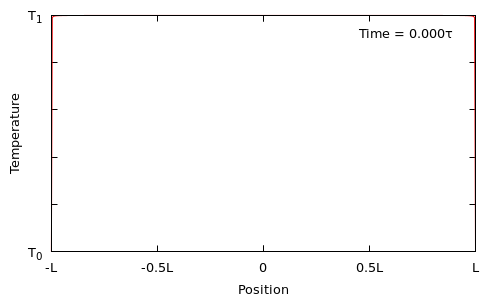
Same as before, but covering only the early stages, from $t=0$ to $t=0.2$ at greater temporal resoluion.

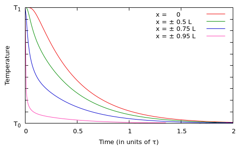
Temperature as function of time, at four different locations along the rod.