Terrain Generation: River Networks
A while back, I looked at the Diamond-Square Algorithm for terrain generation. That is a purely procedural algorithm that only attempts to generate realistic looking landscapes, without trying to model any physical or geological processes. By contrast, we will now look at an algorithm to generate realistic river networks, which is based on a (simplified) model of geological erosion.
The algorithm operates on a two-dimensional square grid. It consists of two parts: in the first, it models the erosion process. In the second, it identifies rivers and streams in the terrain created by the erosion process.
The Erosion Process
The algorithm proceeds as follows.
- Initialize the grid to have a small (typically unit) constant slope in y-direction. In the x-direction, impose periodic boundary conditions on the grid.
- Place a unit of precipitation on a random grid cell.
- Downhill Flow: Randomly select one of the neighboring cells, and let the precipitation flow there. The probability for selecting a cell is based on the height difference $\Delta h = h_i - h_0$ between the height $h_0$ of the current cell and the height $h_i$ of the neighboring cell $i$, as follows: $$ p(i) = \begin{cases} \tfrac{1}{N} e^{ -E \Delta h_i} & \qquad \text{if $\Delta h_i < 0$} \\ 0 & \qquad \text{otherwise} \end{cases} $$ Here, $E \approx 0.05$ is a constant, and $N = \sum_\text{all neighbors} e^{-E \Delta h_i}$ ensures that the probabilities add up to unity. The choice of probabilities guarantees that water will never flow uphill.
- Continue the process until the flow reaches the edge of the grid.
- Erosion: Reduce the height of each visited cell by a constant amount $D \approx 10$. Notice that this process does not conserve material; it is assumed that the eroded substance simply “vanishes”.
- Mudslides: If the height difference $\Delta h$ between any two neighboring cells exceeds a constant value $M \approx 2000$, reduce the height of the taller cell by $\Delta h/4$. Continue the process until all neighbor-neighbor height differences are below the threshold. (Again, mudslides are not material-conserving.)
- Go back to step 2, stop if the desired amount of erosion has been achieved. (Typically 10000 precipitation events for a $300 \times 200$ grid.)
Notice that the numerical values of the resulting terrain “heights” will mostly be negative! Also, the relatively large threshold ($M \approx 2000$) for mudslides is not a typo: mudslides are only expected after a significant amount of erosion has occurred.
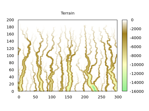
In the figure, the terrain is colored according to its elevation. Notice that the “canyons” carved by erosion and mudslides are much deeper than the initially configured incline.
Identifying Rivers
To identify which cells belong to a “river bed”, we proceed as follows:
- Place a unit of precipitation on each cell of the grid.
- Let it drain downhill, choosing the path of steepest descent. (If there is a tie, break it randomly.)
- Follow the drainage to the end of the grid, without erosion.
- Count how often each cell is visited. Cells that have been visited at least $R \approx 10 \dots 1000$ times are considered part of a river.
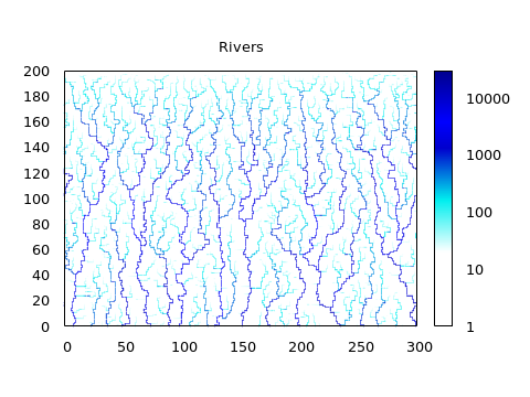
The figure colors individual cells by the amount of drainage they have received in the analysis step, with more frequently visited cells shown in darker color.
Implementation
Although simple, the algorithm can be delicate to implement correctly: a number of edge cases and special conditions must be recognized and treated appropriately. A straightforward implementation of the basic algorithm can be found among the resources — mostly as a starting point for further explorations.
The implementation is intentionally bare-bones, with only the most rudimentary output options, and no support for arbitrary geometries or starting configurations. It would be interesting to consider different starting configurations, for example a central peak with the terrain initially falling off in all directions.
Currently, the implementation only produces data for use in figures, but it does not produce the connected set of coordinates that make up each of the “rivers”. It would be an interesting exercise to follow each river upstream to determine the coordinates that make up the connected graph for each river network.
Resources
This model was described and studied in a paper entitled “Simple model for river network evolution” by Robert L. Leheny, which was published in Physical Review E, Volume 52 (1995), p5610.
The reference implementation: